Fit a negative binomial regression model

Fits a negative binomial GLM (via MASS::glm.nb()) and returns model coefficients on the response scale (exponentiated), randomized quantile residuals (RQR), a Pearson dispersion ratio, and diagnostic plots.

Usage

negbinGLM(
  formula,
  data,
  assessZeroInflation = TRUE,
  maxit = NULL,
  dispersion_threshold = 1.2,
  ...
)

Arguments

formula: A model formula (e.g. y ~ x1 + x2). The response must be a non-negative integer count variable.
data: A data frame containing the variables in formula.
assessZeroInflation: Logical; when TRUE (default), runs a DHARMa simulation-based zero-inflation test after fitting. Issues a warning if significant zero-inflation is detected and adds zi_test to the returned diagnostics. Set to FALSE when calling from countGLM(), which performs its own zero-inflation assessment.
maxit: Optional integer; maximum IWLS iterations passed through as control = stats::glm.control(maxit = maxit). Ignored when the user supplies their own control via ....
dispersion_threshold: Numeric; dispersion ratios above this value are flagged as overdispersed in the diagnostic plot. Default 1.2.
...: Additional arguments passed to MASS::glm.nb().

Value

An object of class c("negbinGLM", "countGLMfit"), a list with:

call

The matched call.

model

The underlying MASS::glm.nb fit object.

summary

The result of summary() on the fitted model.

theta

The estimated negative binomial dispersion parameter (smaller values indicate more overdispersion).

coefficients

A data frame with columns term, exp.coef, lower.95, upper.95 (all on the response/exponentiated scale).

diagnostics

A list with:

rqr: Numeric vector of randomized quantile residuals.
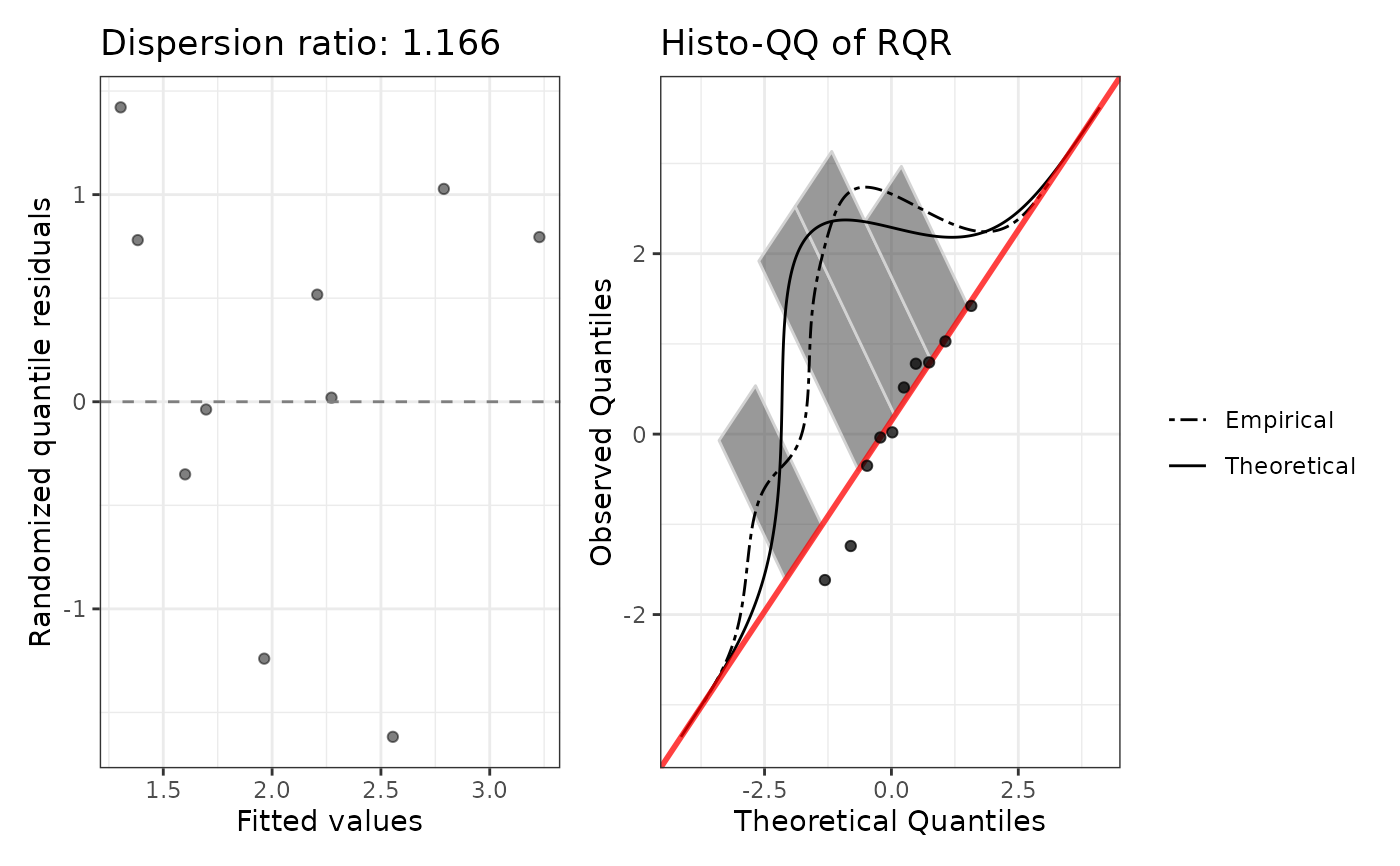
dispersion_ratio: Pearson chi-squared / df.residual.
plot: Patchwork ggplot: fitted vs RQR and histo-QQ.
r2_plot: Squared Pearson residuals vs fitted values.
zi_test: When assessZeroInflation = TRUE, a list with detected (logical), p_value (numeric), and plot (ggplot histogram of DHARMa simulated zero proportions vs observed). NULL when assessZeroInflation = FALSE.

aic

AIC of the fitted model.

bic

BIC of the fitted model.

Details

Coefficient interpretation: Negative binomial regression models the log of the expected count. Exponentiating a coefficient gives the multiplicative change in the expected count for a one-unit increase in the predictor.

When to use: Negative binomial is appropriate when count data show overdispersion (variance > mean). A Pearson dispersion ratio from poissonGLM() substantially above 1 (rule of thumb: > 1.5) is a common signal. The negative binomial adds a free parameter theta to model this extra variance. For count data with complex variance structures, consider tweedieGLM(). If zero-inflation is also detected, consider zeroinflNegbinGLM().

Examples

df <- data.frame(
  y  = c(0L, 1L, 2L, 3L, 5L, 0L, 2L, 4L, 1L, 3L),
  x1 = c(1.2, -0.4, 0.8, -1.1, 2.0, 0.3, -0.9, 1.5, -0.2, 0.7)
)
fit <- negbinGLM(y ~ x1, data = df)
#> Warning: Count component: 8 events (y > 0) for 1 predictor(s) (8.0 per predictor). At least 10 events per predictor is recommended.
#> Warning: iteration limit reached
#> Warning: iteration limit reached
print(fit)
#> 
#> Call:
#> negbinGLM(formula = y ~ x1, data = df)
#> 
#> Model family: negbinGLM 
#> 
#> Coefficients (on response scale):
#>         term exp.coef lower.95 upper.95 p.value stars
#>  (Intercept)   1.7989   1.0683   3.0291  0.0272     *
#>           x1   1.3396   0.8571   2.0936  0.1994      
#> 
#> Dispersion ratio: 1.1657
#> AIC: 41.02
plot(fit)