Fit a zero-inflated negative binomial regression model

Fits a zero-inflated negative binomial model (via pscl::zeroinfl()) with separate count and zero-inflation components. Returns coefficients on the response scale, randomized quantile residuals, a dispersion ratio, and a diagnostic plot.

Usage

zeroinflNegbinGLM(
  formula,
  data,
  ziformula = NULL,
  maxit = NULL,
  dispersion_threshold = 1.2,
  ...
)

Arguments

formula: A model formula for the count component (e.g. y ~ x1 + x2). The response must be a non-negative integer count.
data: A data frame containing the variables in formula (and ziformula if provided).
ziformula: A one-sided formula for the zero-inflation component (e.g. ~ x1). When NULL (default), the same right-hand side as formula is used for both components. Use ~ 1 for an intercept-only zero-inflation model.
maxit: Optional integer; maximum optimizer iterations passed through as control = pscl::zeroinfl.control(maxit = maxit). Ignored when the user supplies their own control via ....
dispersion_threshold: Numeric; dispersion ratios above this value are flagged as overdispersed in the diagnostic plot. Default 1.2.
...: Additional arguments passed to pscl::zeroinfl().

Value

An object of class c("zeroinflNegbinGLM", "zeroinflGLMfit", "countGLMfit"), a list with:

call

The matched call.

model

The underlying pscl::zeroinfl fit object.

theta

The estimated negative binomial dispersion parameter.

coefficients

A list with two data frames, each with columns term, exp.coef, lower.95, upper.95:

count: Exponentiated coefficients for the count component.
zero: Exponentiated coefficients for the zero-inflation component.

summary

The result of summary() on the fitted model.

diagnostics

A list with rqr, dispersion_ratio, and plot (see poissonGLM() for details).

aic

AIC of the fitted model.

bic

BIC of the fitted model.

Details

Coefficient interpretation:

Count component: exponentiating a coefficient gives the multiplicative change in the expected count among non-structural-zero observations, for a one-unit increase in the predictor, adjusting for simultaneous linear changes in other predictors. For example, 1.5 means a 50% higher expected count.
Zero component: exponentiating a coefficient gives the multiplicative change in the odds of being a structural zero (vs. entering the count process) for a one-unit increase in the predictor.

When to use: Zero-inflated negative binomial handles both excess zeros and overdispersion in the non-zero counts. Prefer this over zeroinflPoissonGLM() when the non-zero counts remain overdispersed. For count data with complex variance structures and excess zeros, consider zeroinflTweedieGLM().

Examples

df <- data.frame(
  y  = c(0L, 0L, 0L, 1L, 2L, 0L, 3L, 0L, 1L, 0L),
  x1 = c(1.2, -0.4, 0.8, -1.1, 2.0, 0.3, -0.9, 1.5, -0.2, 0.7)
)
fit <- zeroinflNegbinGLM(y ~ x1, data = df)
#> Warning: Count component: 4 events (y > 0) for 1 predictor(s) (4.0 per predictor). At least 10 events per predictor is recommended.
#> Warning: Zero-inflation component: 6 zeros for 1 predictor(s) (6.0 per predictor). At least 10 zeros per ZI predictor is recommended.
print(fit)
#> 
#> Call:
#> zeroinflNegbinGLM(formula = y ~ x1, data = df)
#> 
#> Model family: zeroinflNegbinGLM 
#> 
#> Count component (exponentiated coefficients):
#>         term exp.coef lower.95 upper.95 p.value stars
#>  (Intercept)   1.3408   0.4922   3.6523  0.5663      
#>           x1   0.9433   0.4383   2.0304  0.8814      
#> 
#> Zero-inflation component (exponentiated coefficients):
#>         term exp.coef lower.95 upper.95 p.value stars
#>  (Intercept)   0.6737   0.0820   5.5325  0.7131      
#>           x1   2.1030   0.4077  10.8486  0.3745      
#> 
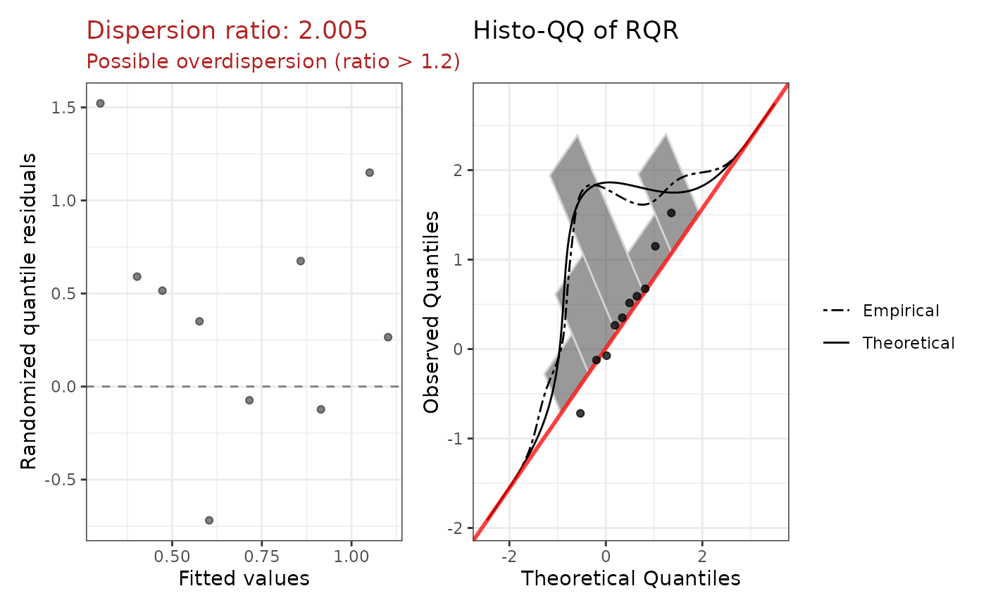
#> Dispersion ratio: 2.0053
#> AIC: 31.60
plot(fit)


# Intercept-only zero component:
fit2 <- zeroinflNegbinGLM(y ~ x1, data = df, ziformula = ~ 1)
#> Warning: Count component: 4 events (y > 0) for 1 predictor(s) (4.0 per predictor). At least 10 events per predictor is recommended.