Fit a quasi-Poisson regression model

Fits a quasi-Poisson GLM via stats::glm(family = quasipoisson()) and returns exponentiated coefficients with quasi-likelihood Wald 95% CIs, the estimated dispersion parameter (phi), Pearson dispersion ratio, and diagnostic plots. Quasi-Poisson shares the Poisson mean structure but estimates a free scale parameter so that Var(Y) = phi * mu.

Usage

quasiPoissonGLM(formula, data, maxit = NULL, dispersion_threshold = 1.2, ...)

Arguments

formula

A model formula (e.g. y ~ x1 + x2). The response must be a non-negative integer count variable.

data

A data frame containing the variables in formula.

maxit

Optional integer; maximum IWLS iterations passed through as control = stats::glm.control(maxit = maxit). Ignored when the user supplies their own control via ....

dispersion_threshold

Numeric; dispersion ratios above this value are flagged as overdispersed in the diagnostic plot. Default 1.2.

...

Additional arguments passed to stats::glm().

Value

An object of class c("quasiPoissonGLM", "countGLMfit"), a list with:

call

The matched call.

model

The underlying stats::glm fit object.

summary

The result of summary() on the fitted model.

phi

The estimated quasi-likelihood dispersion parameter (summary(fit)$dispersion).

coefficients

A data frame with columns term, exp.coef, lower.95, upper.95, p.value, and stars. Standard errors (and hence CIs and p-values) are inflated by sqrt(phi) relative to a Poisson fit.

diagnostics

A list with:

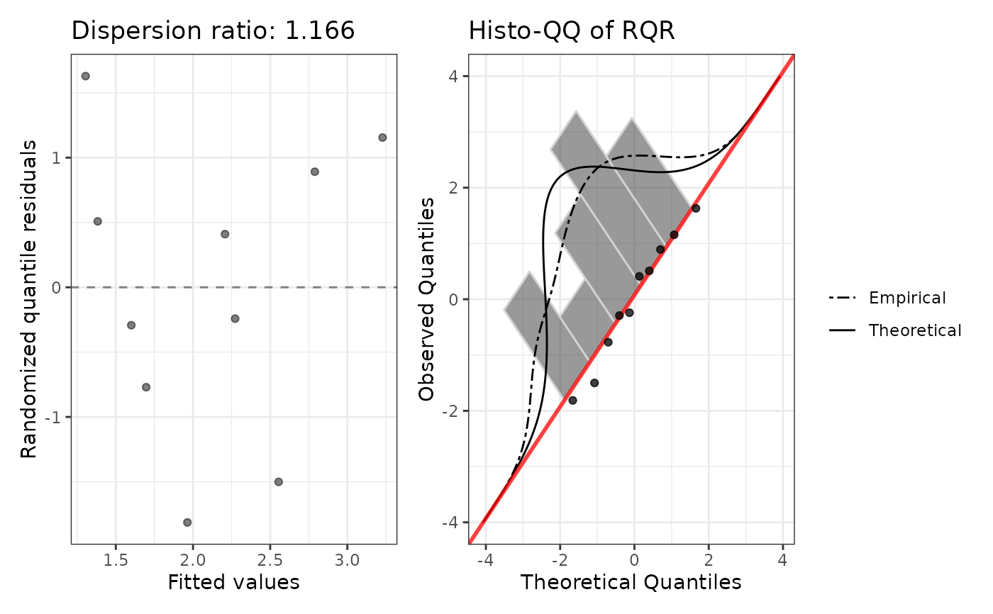
rqr

Numeric vector of randomized quantile residuals, computed from the Poisson CDF evaluated at the fitted means (quasi-Poisson shares the Poisson mean structure).

dispersion_ratio

Pearson chi-squared / df.residual, equal to phi.

plot

Patchwork ggplot: fitted vs RQR and histo-QQ. The dispersion-ratio label in the title equals phi.

r2_plot

Squared Pearson residuals vs fitted values.

aic

NA_real_. Quasi-likelihood fits do not have a proper likelihood, so AIC is undefined.

bic

NA_real_. BIC is also undefined for quasi-likelihood fits.

Details

Coefficient interpretation: Identical to Poisson regression; exponentiating a coefficient gives the multiplicative change in the expected count for a one-unit increase in the predictor. The point estimates match poissonGLM() exactly — only the standard errors differ.

When to use: Quasi-Poisson is appropriate when a Poisson fit shows mild-to-moderate overdispersion that appears constant across the range of fitted values — i.e. the squared Pearson residuals form a roughly flat cloud with mean phi > 1, rather than fanning out with the fitted mean (which would motivate negbinGLM()). countGLM() automatically fits quasi-Poisson when the Poisson dispersion ratio exceeds 1.2 and the r² vs fitted plot is approximately flat above 1.

No AIC/BIC: Because quasi-Poisson is a quasi-likelihood method, AIC and BIC are not defined and are returned as NA. Quasi-Poisson therefore does not participate in the likelihood-based comparison performed by countGLM(); it is reported alongside the main comparison when flagged.

See also

poissonGLM(), negbinGLM(), tweedieGLM(), countGLM(), stats::glm()

Examples

df <- data.frame(
  y  = c(0L, 1L, 2L, 3L, 5L, 0L, 2L, 4L, 1L, 3L),
  x1 = c(1.2, -0.4, 0.8, -1.1, 2.0, 0.3, -0.9, 1.5, -0.2, 0.7)
)
fit <- quasiPoissonGLM(y ~ x1, data = df)
#> Warning: Count component: 8 events (y > 0) for 1 predictor(s) (8.0 per predictor). At least 10 events per predictor is recommended.
print(fit)
#> 
#> Call:
#> quasiPoissonGLM(formula = y ~ x1, data = df)
#> 
#> Model family: quasiPoissonGLM
#> 
#> Coefficients (on response scale):
#>         term exp.coef lower.95 upper.95 p.value stars
#>  (Intercept)   1.7989   0.9279   3.4873  0.0750     .
#>           x1   1.3396   0.7597   2.3622  0.2687      
#> 
#> Dispersion (phi): 1.1658
#> Dispersion ratio: 1.1658
#> AIC: NA (quasi-likelihood)
plot(fit)